surveyjoin

This vignette represents an introduction to using the surveyjoin package. We’ll load the package, along with dplyr and ggplot2 for data manipulation and plotting.

library(surveyjoin)
library(dplyr)
#> 
#> Attaching package: 'dplyr'
#> The following objects are masked from 'package:stats':
#> 
#>     filter, lag
#> The following objects are masked from 'package:base':
#> 
#>     intersect, setdiff, setequal, union
library(ggplot2)
#> Warning: package 'ggplot2' was built under R version 4.3.2

The surveyjoin package contains several processing functions that will download the survey data files locally, and create a connection to the SQLite database. The cache_data() function pulls data from a public Github repository, and needs to be only run every time the raw data is refreshed (a new year of survey data becomes available).

cache_data()
load_sql_data()

If you try to run these functions too many times in an hour, the Github API will timeout, and the load_sql_data() function will work with the files that are already locally cached. You can check the versions (dates) on individual files with

data_version()

Several helper functions have been included to provide more information on the metadata, survey shapefiles, and links to the original data. Each of these returns a dataframe with a URL for each of our three regions (“afsc”, “pbs”, “nwfsc”).

get_metadata()
get_shapefiles()
get_rawdata()

Additionally, we can look at the table of species names (common, scientific, itis) that are included.

get_species()

The core function of the package is get_data. This allows for querying by species (using common names - “common”, scientific names - “scientific”, or ITIS identifiers - “itis_id”), regions, surveys, or years – each of these may be a single value or vector of values. We could get data for sablefish from all Alaska surveys in the the last decade with

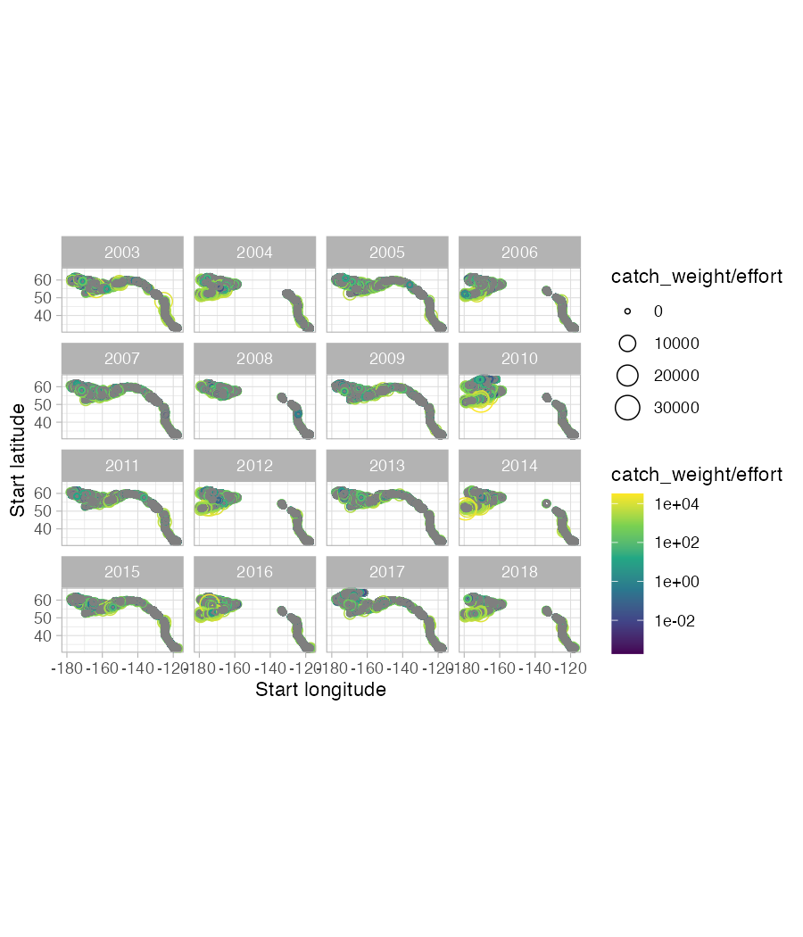
d <- get_data(common = "sablefish", years = 2013:2023, regions = "afsc")

As a second example, we could get data coastwide for Arrowtooth flounder and plot it with the following code. We’ll constrain it to years 2003-2018 for plotting purposes (though the earliest year of data is 1980).

d <- get_data(common = "arrowtooth flounder", years = 2003:2018)

g <- d |>
  ggplot(aes(
    lon_start,
    lat_start,
    colour = catch_weight / effort,
    size = catch_weight / effort
  )) +
  geom_point(pch = 21) +
  facet_wrap(~year) +
  scale_colour_viridis_c(trans = "log10") +
  theme_light() +
  coord_fixed() +
  xlab("Start longitude") +
  ylab("Start latitude")

ggsave(g,
  filename = "map-example.png",
  width = 6, height = 7, dpi = 150
)

Additional information on specific species can be found in our species dictionary

data("spp_dictionary")

And the full list of survey names can be found with

get_survey_names()
#>                 survey region
#> 1     Aleutian Islands   afsc
#> 2       Gulf of Alaska   afsc
#> 3   eastern Bering Sea   afsc
#> 4  northern Bering Sea   afsc
#> 5     Bering Sea Slope   afsc
#> 6          NWFSC.Combo  nwfsc
#> 7          NWFSC.Shelf  nwfsc
#> 8        NWFSC.Hypoxia  nwfsc
#> 9        NWFSC.Hypoxia  nwfsc
#> 10           Triennial  nwfsc
#> 11             SYN QCS    pbs
#> 12              SYN HS    pbs
#> 13            SYN WCVI    pbs
#> 14            SYN WCHG    pbs